Working with graphs#
This notebook gives a few examples how Pyrosm can be used together with Python network analysis libraries. Before starting, ensure that you have read the basic documentation about how to export graphs with Pyrosm.
Contents:
Calculate the catchment areas of hospitals in Estonia with
pyrosm + igraph.Calculate the job accessibility in Helsinki Region with
pyrosm + pandarm
Note
The idea of this page is not to give a comprehensive overview of all the possibilities that you can do with these network analysis libraries, but to just give you a bit of idea what can be done. You can get more detailed and further information from the documentation of the packages themselves.
Integrating routing or network analysis functionalities is not planned for Pyrosm. There is a separate Python project called
cafeinthat will be built on top ofpyrosmincluding different routing and network analysis functionalities (will become available in 2021).
Export street networks to graph#
If you want to analyze the street networks using your favourite network analysis library, you can export the street network from Pyrosm into a graph (new in version 0.6.0). Supported graphs are iGraph, NetworkX (compatible with OSMnx), Pandarm and Pandana. Those libraries provide numerous possibilities to analyze different properties of the graph (e.g. centrality) or conduct e.g. shortest path analysis to find the fastest (or shortest) route from a location to another. Notice that the numerous algorithms provided by these libraries are not going to be integrated into Pyrosm, but you can easily export the graphs to these libraries and continue working with them.
Exporting the network into a graph can be done as follows:
Retrieve the graph elements (nodes and edges) from a given OSM network by specifying
nodes=Truein theosm.get_network()function.Use
osm.to_graph()function to convert the nodes and edges into a graph.The output graph type can be specified with
graph_typeparameter. Available types are:"igraph"(default),"networkx","pandarm"and"pandana"(deprecated; use"pandarm").
Following sections show how to do this in practice.
What is a graph? (a super short intro)
Graphs are, in principle, quite simple data structures consisting of:
nodes (e.g. intersections on a street, or a person in social network), and
edges (a link that connects the nodes to each other)
A simple graph could look like this:
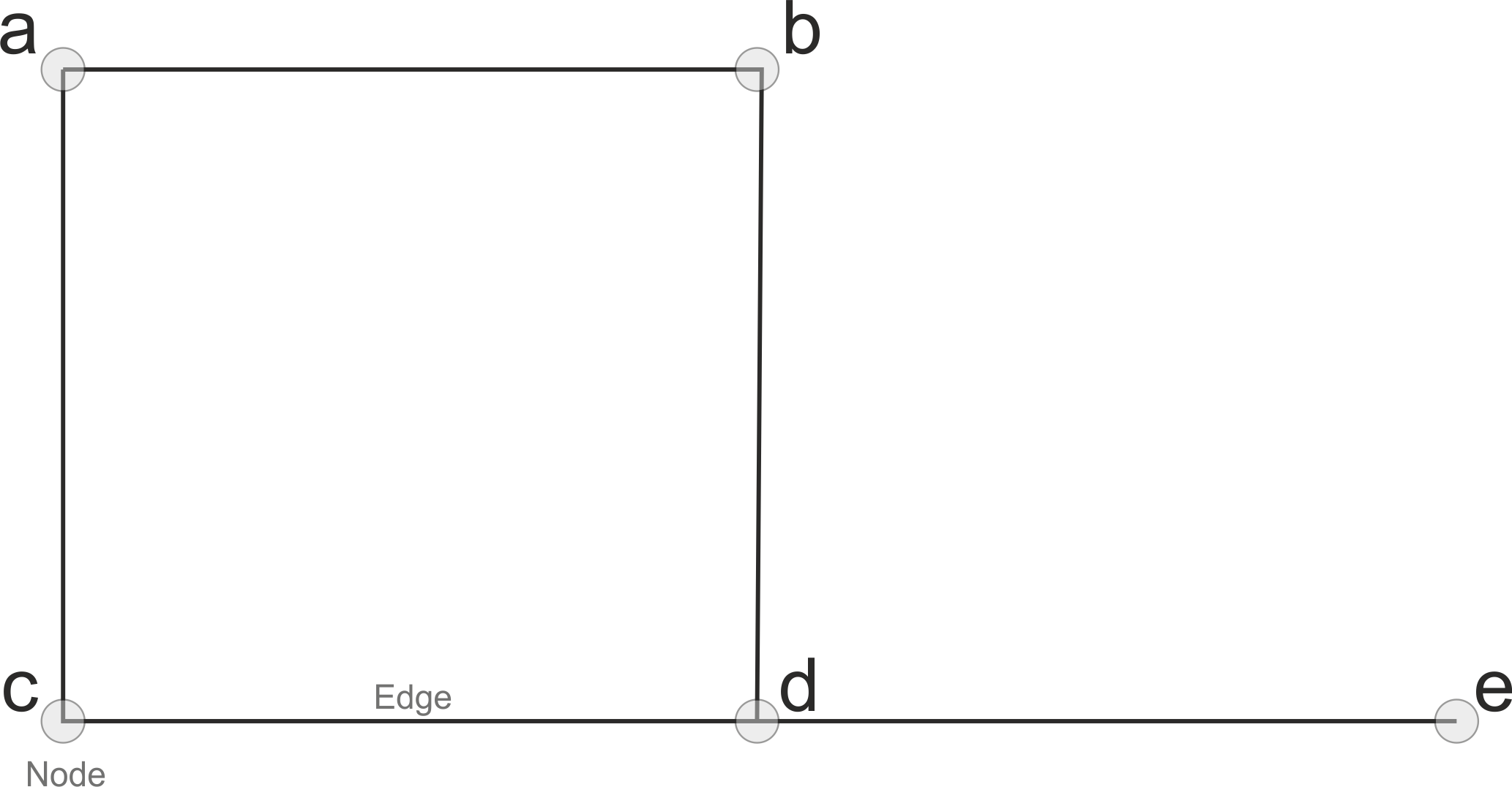 Simple graph with five nodes and edges between them.
Graph can be directed or undirected, which basically determines whether the roads can be travelled to any direction or whether the travel direction is restricted to certain direction (e.g. a one-way-street). A directed graph looks something like this:
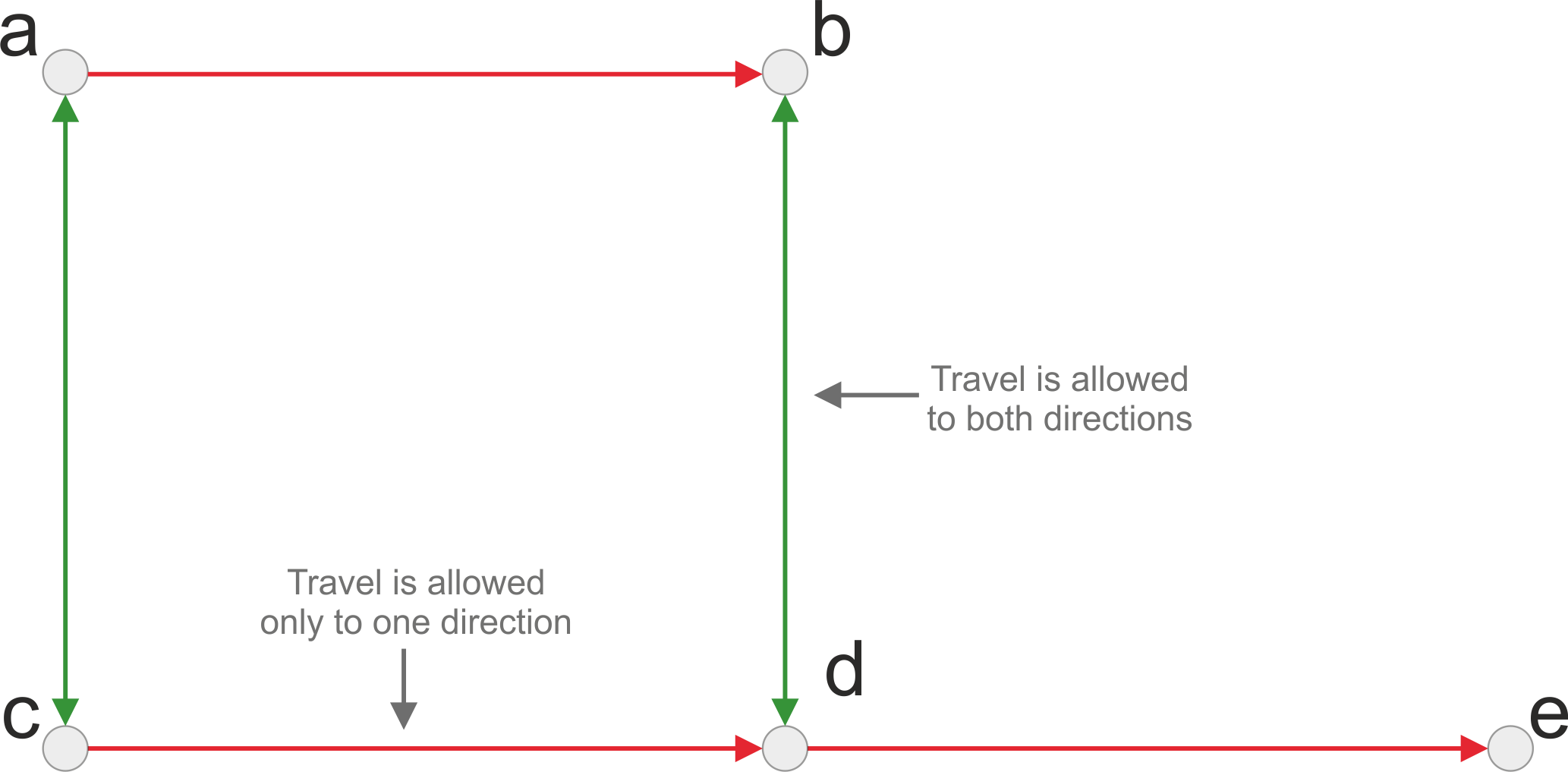 Directed graph.
Notes about Pyrosm graph building#
Pyrosm will always create a directed graph when exporting the street network to graph (works similarly for all libraries).
When exporting network that is used for driving (i.e.
network_type="driving"), pyrosm considers the oneway restrictions that are defined inonewaycolumn in the data.With “walking”, “cycling” and “all”, pyrosm creates a bidirectional graph, meaning that the travel is allowed to both directions.
By default, Pyrosm will only keep connected edges in the output graph (largest strongly connected component). This means that all “isolated islands” of the network will be filtered out because those cannot be reached from other parts of the network (you can change this behavior by specifying
retain_all=True, see further info).When constructing the graph, all road segments are kept separate to ensure good connectivity. You can simplify the graph (reducing its size) by passing
simplify=Truetoto_graph(): this removes interstitial degree-2 nodes and merges each chain of segments between two intersections into a single edge, while keeping the full geometry. It works for every graph type and is equivalent to OSMnx’s graph simplification. See the Simplify the graph section below.
Read nodes and edges (first step)#
The first step that needs to be done is to read the nodes and edges from the graph:
from pyrosm import OSM, get_data

# Initialize reader
osm = OSM(get_data("test_pbf"))

# Read nodes and edges of the 'driving' network
nodes, edges = osm.get_network(nodes=True, network_type="driving")

# Plot nodes and edges on a map
ax = edges.plot(figsize=(6,6), color="gray")
ax = nodes.plot(ax=ax, color="red", markersize=2.5)
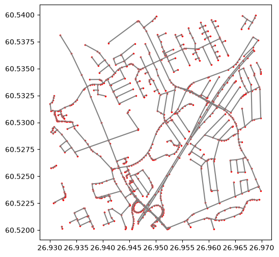
The map shows the nodes (red color) and edges (gray color) which connect the nodes to each other (thus constructing the network).
When parsing the nodes, two extra columns (u and v) are added to the GeoDataFrame. These columns specify the source (u) and target (u) nodes for each edge (also commonly called as from- and to-ids):
# Show the last 5 columns of the first 5 rows in edges
edges.iloc[:5, -5:]
| osm_type | geometry | u | v | length | |
|---|---|---|---|---|---|
| 0 | way | LINESTRING (26.9431 60.5258, 26.94295 60.52596) | 36156596 | 2316826913 | 20.096 |
| 1 | way | LINESTRING (26.94295 60.52596, 26.94261 60.52639) | 2316826913 | 3735963133 | 51.356 |
| 2 | way | LINESTRING (26.94261 60.52639, 26.94132 60.52804) | 3735963133 | 277446336 | 196.370 |
| 3 | way | LINESTRING (26.94132 60.52804, 26.94108 60.52835) | 277446336 | 3730253796 | 36.410 |
| 4 | way | LINESTRING (26.94108 60.52835, 26.93975 60.52998) | 3730253796 | 277446337 | 195.452 |
The u and v values have corresponding data in the nodes GeoDataFrame (column id):
# 'id' column here corresponds to the 'u' and 'v' values in edges GeoDataFrame
nodes.head()
| version | lat | visible | lon | timestamp | tags | changeset | id | geometry | |
|---|---|---|---|---|---|---|---|---|---|
| 0 | 4 | 60.525798 | False | 26.943103 | 1369300078 | None | 0 | 36156596 | POINT (26.9431 60.5258) |
| 1 | 1 | 60.525962 | False | 26.942948 | 1369300072 | {'highway': 'crossing'} | 0 | 2316826913 | POINT (26.94295 60.52596) |
| 2 | 1 | 60.526393 | False | 26.942611 | 1441800372 | None | 0 | 3735963133 | POINT (26.94261 60.52639) |
| 3 | 4 | 60.528041 | False | 26.941323 | 1282588818 | None | 0 | 277446336 | POINT (26.94132 60.52804) |
| 4 | 1 | 60.528345 | False | 26.941076 | 1441438154 | None | 0 | 3730253796 | POINT (26.94108 60.52835) |
Export to iGraph#
Python’s iGraph library is used by default when exporting the nodes and edges to graph. iGraph is a good choice for analyzing large graphs (such as the street networks parsed with Pyrosm) as it is faster and more memory efficient than e.g. NetworkX.
To export the nodes and edges into directed graph that can be used with igraph library, you pass the data into osm.to_graph() -function:
from pyrosm import OSM, get_data
osm = OSM(get_data("test_pbf"))
nodes, edges = osm.get_network(nodes=True, network_type="driving")

# Create a graph for igraph from nodes and edges
G = osm.to_graph(nodes, edges)
G
<igraph.Graph at 0x1755d2e50>
As an output, you get a directed igraph.Graph object that can be used for further analysis using the various functionalities of igraph.
See all available parameters of to_graph() from here and usage examples from working with graphs.
Export to NetworkX / OSMnx#
NetworkX and OSMnx (focusing on street networks) are two widely used network analysis libraries for Python. Exporting the OSM street network to these libraries is easy. You just need to specify graph_type="networkx" when calling the to_graph() function:
from pyrosm import OSM, get_data
osm = OSM(get_data("test_pbf"))
nodes, edges = osm.get_network(nodes=True, network_type="driving")

# Export the nodes and edges to NetworkX graph
G = osm.to_graph(nodes, edges, graph_type="networkx")
G
<networkx.classes.multidigraph.MultiDiGraph at 0x1082cb620>
As an output, you get a directed networkx MultiDiGraph object that can be used for further analysis using either NetworkX or OSMnx.
See all available parameters of to_graph() from here and usage examples from working with graphs.
Note
By default, when exporting to networkx, the edge and node attributes are named in such a way that you can directly start using osmnx functionalities. Also a column key (with value 0) is automatically added to the edge table to make the data compatible with osmnx.
If you want to disable these modifications, specify osmnx_compatible=False when exporting the data to graph, i.e:
G2 = osm.to_graph(nodes, edges, graph_type="networkx", osmnx_compatible=False)
Export to Pandarm#
Pandarm (the maintained, NumPy 2-compatible fork of Pandana) is a Python library for conducting accessibility/reachability analysis using the contraction hierarchies algorithm. It has useful functionalities to conduct more specific queries such as “find me all restaurants that are within 500 meters from given locations (e.g. buildings)”.
Exporting the OSM street network to Pandarm works in a similar manner as with the previous ones. By specifying graph_type="pandarm" for the to_graph() function, the output will be a pandarm graph. In addition, you can specify with pandana_weights -parameter which columns in your edges data is used as edge weights in the graph. By default length column is used but you can add any other numerical column as an edge weight (you can use multiple weights in the same graph):
Note
graph_type="pandana" is still accepted for backwards compatibility, but pandana is deprecated (unmaintained and incompatible with NumPy 2 on Windows) and will be removed in a future release. Use "pandarm" instead.
from pyrosm import OSM, get_data
osm = OSM(get_data("test_pbf"))
nodes, edges = osm.get_network(nodes=True, network_type="driving")

# Export the nodes and edges to Pandarm graph
G = osm.to_graph(nodes, edges, graph_type="pandarm", pandana_weights=["length"])
G
Generating contraction hierarchies with 10 threads.
Setting CH node vector of size 768
Setting CH edge vector of size 1490
Range graph removed 1360 edges of 2980
. 10% . 20% . 30% . 40% . 50% . 60% . 70% . 80% . 90% . 100%
 100%
/Users/tenkanh2/Library/CloudStorage/OneDrive-AaltoUniversity/Documents/codes/uni/pyrosm/pyrosm/graphs.py:411: UserWarning: No CRS was passed to geometry input; assuming geographic coordinates
  return _create_pandarm_graph(nodes, edges, from_id_col, to_id_col, weight_cols)
<pandarm.network.Network at 0x175d92510>
As an output, you get a directed pandarm Network object that can be used for further analysis using pandarm.
See all available parameters of to_graph() from here and usage examples from working with graphs.
to_graph parameters explained#
to_graph() function has multiple parameters that can be adjusted. Below you can read all available parameters, and their explanations:
from pyrosm import OSM, get_data
osm = OSM(get_data("test_pbf"))

# To see all available parameters and their explanations, simply call help
help(osm.to_graph)
Help on function to_graph in module pyrosm.pyrosm:

to_graph(
    nodes,
    edges,
    graph_type='igraph',
    direction='oneway',
    from_id_col='u',
    to_id_col='v',
    edge_id_col='id',
    node_id_col='id',
    force_bidirectional=False,
    network_type=None,
    retain_all=False,
    osmnx_compatible=True,
    pandana_weights=['length'],
    simplify=False,
    simplify_kwargs=None
)
    Export OSM network to routable graph. Supported output graph types are:

      - "igraph" (default),
      - "networkx",
      - "pandarm",
      - "pandana" (deprecated; use "pandarm")

    For walking, the output graph will be bidirectional by default
    (i.e. travel along the street is allowed to both directions). For driving
    and cycling, one-way streets are taken into account by default and the
    travel is restricted based on the rules in OSM data (the "oneway"
    attribute; cycling additionally honours "oneway:bicycle" so that
    contraflow cycling on one-way streets is modelled correctly).

    Set ``simplify=True`` to topologically simplify the graph before export:
    interstitial degree-2 nodes are removed and each intersection-to-intersection
    chain is collapsed into a single edge that keeps the full geometry. This
    reduces the graph size while preserving routing distances and is equivalent to
    ``osmnx.simplification.simplify_graph``.

    Parameters
    ----------

    nodes : GeoDataFrame
        GeoDataFrame containing nodes of the road network.
        Note: Use `osm.get_network(nodes=True)` to retrieve both the nodes and edges.

    edges : GeoDataFrame
        GeoDataFrame containing the edges of the road network.

    graph_type : str
        Type of the output graph. Available graphs are:
          - "igraph" --> returns an igraph.Graph -object.
          - "networkx" --> returns a networkx.MultiDiGraph -object.
          - "pandarm" --> returns a pandarm.Network -object.
          - "pandana" --> returns a pandana.Network -object.
            (deprecated: pandana is unmaintained and incompatible with
            NumPy 2 on Windows; use "pandarm" instead. Will be removed in
            a future release.)

    direction : str
        Name for the column containing information about the allowed driving directions

    from_id_col : str
        Name for the column having the from-node-ids of edges.

    to_id_col : str
        Name for the column having the to-node-ids of edges.

    edge_id_col : str
        Name for the column having the unique id for edges.

    node_id_col : str
        Name for the column having the unique id for nodes.

    force_bidirectional : bool
        If True, all edges will be created as bidirectional (allow travel to both directions).

    network_type : str (optional)
        Network type for the given data. Determines how the graph will be constructed.
        The network type is typically extracted automatically from the metadata of
        the edges/nodes GeoDataFrames. This parameter can be used if this metadata is not
        available for a reason or another. By default, a bidirectional graph is created for walking and all,
        and a directed graph for driving and cycling (oneway streets are taken into account;
        cycling additionally honours oneway:bicycle for contraflow).
        Possible values are: 'walking', 'cycling', 'driving', 'driving+service', 'all'.

    retain_all : bool
        if True, return the entire graph even if it is not connected.
        otherwise, retain only the connected edges.

    osmnx_compatible : bool (default True)
        if True, modifies the edge and node-attribute naming to be compatible with OSMnx
        (allows utilizing all OSMnx functionalities).
        NOTE: Only applicable with "networkx" graph type.

    pandana_weights : list
        Columns that are used as weights when exporting to Pandana graph. By default uses "length" column.

    simplify : bool (default False)
        If True, topologically simplify the graph before export: interstitial
        nodes that only carry geometry (degree-2 pass-throughs) are removed and
        each chain between intersections/endpoints is collapsed into a single edge
        that keeps the full geometry. Edge ``length`` is summed along the chain and
        the merged geometry runs from ``u`` to ``v``. The result is equivalent to
        ``osmnx.simplification.simplify_graph``. See
        ``pyrosm.graph_simplify.simplify_graph`` for details.

    simplify_kwargs : dict (optional)
        Keyword arguments forwarded to ``pyrosm.graph_simplify.simplify_graph``
        when ``simplify=True``, e.g. ``edge_attrs_differ`` (do not merge across a
        change in the listed columns), ``node_attrs_include`` (keep the listed
        nodes as endpoints), ``remove_rings``, ``track_merged`` or ``length_cols``.
Simplify the graph#
When the nodes and edges are parsed, every individual road segment is kept as its own row so that the graph stays fully connected. For many analyses you don’t need that detail — you care about the intersections and the links between them. Passing simplify=True to to_graph() collapses the network topologically: interstitial degree-2 nodes (which only describe the shape of a road) are removed, and each chain of segments between two intersections is merged into a single edge that keeps the full geometry. Edge length is summed along the chain, so routing distances are preserved.
This is equivalent to OSMnx’s graph simplification and follows the method described in Boeing, G. (2025), “Topological Graph Simplification Solutions to the Street Intersection Miscount Problem”, Transactions in GIS, 29: e70037 (https://doi.org/10.1111/tgis.70037). It works for every output graph type (igraph, networkx, pandarm).
from pyrosm import OSM, get_data
osm = OSM(get_data("test_pbf"))
nodes, edges = osm.get_network(nodes=True, network_type="driving")

# Full graph vs. topologically simplified graph
G_full = osm.to_graph(nodes, edges, simplify=False)
G_simple = osm.to_graph(nodes, edges, simplify=True)

print(f"Full:       {G_full.vcount()} nodes, {G_full.ecount()} edges")
print(f"Simplified: {G_simple.vcount()} nodes, {G_simple.ecount()} edges")
Full:       768 nodes, 1490 edges
Simplified: 268 nodes, 577 edges
The simplification can be fine-tuned with simplify_kwargs. For example, prevent a chain from merging across a change in road class so that, say, a primary and a residential stretch stay as separate edges:
G = osm.to_graph(
    nodes, edges,
    simplify=True,
    simplify_kwargs={"edge_attrs_differ": ["highway"]},
)
Other options include node_attrs_include (keep specific nodes as intersections), remove_rings, and track_merged.
Find shortest path with Pyrosm + NetworkX + OSMnx#
This tutorial shows how to construct simple shortest path routing between selected source and destination addresses using NetworkX and OSMnx. Pyrosm is used for extracting the data from OSM PBF file and constructing the graph, while NetworkX provides the basic network analysis capabilities and OSMnx provides many useful functionalities that makes it easy to work with street networks.
from pyrosm import OSM, get_data
import osmnx as ox

# Initialize the reader
osm = OSM(get_data("helsinki_pbf"))

# Get all walkable roads and the nodes
nodes, edges = osm.get_network(nodes=True)

# Check first rows in the edge
edges.head()
| access | bicycle | bridge | cycleway | est_width | foot | footway | highway | int_ref | lanes | ... | width | id | timestamp | version | tags | osm_type | geometry | u | v | length | |
|---|---|---|---|---|---|---|---|---|---|---|---|---|---|---|---|---|---|---|---|---|---|
| 0 | NaN | NaN | NaN | NaN | NaN | NaN | NaN | unclassified | NaN | 2 | ... | NaN | 4236349 | 1380031970 | 21 | {"visible":false,"name:fi":"Erottajankatu","na... | way | LINESTRING (24.94327 60.16651, 24.94337 60.16644) | 1372477605 | 292727220 | 9.370 |
| 1 | NaN | NaN | NaN | NaN | NaN | NaN | NaN | unclassified | NaN | 2 | ... | NaN | 4236349 | 1380031970 | 21 | {"visible":false,"name:fi":"Erottajankatu","na... | way | LINESTRING (24.94337 60.16644, 24.9434 60.16641) | 292727220 | 2394117042 | 4.499 |
| 2 | NaN | NaN | NaN | NaN | NaN | NaN | NaN | unclassified | NaN | 2 | ... | NaN | 4243035 | 1543430213 | 12 | {"visible":false,"name:fi":"Korkeavuorenkatu",... | way | LINESTRING (24.94567 60.16767, 24.94567 60.16763) | 296250563 | 2049084195 | 4.174 |
| 3 | NaN | NaN | NaN | NaN | NaN | NaN | NaN | unclassified | NaN | 2 | ... | NaN | 4243035 | 1543430213 | 12 | {"visible":false,"name:fi":"Korkeavuorenkatu",... | way | LINESTRING (24.94567 60.16763, 24.94569 60.16744) | 2049084195 | 60072359 | 21.692 |
| 4 | NaN | NaN | NaN | NaN | NaN | NaN | NaN | unclassified | NaN | 2 | ... | NaN | 4243035 | 1543430213 | 12 | {"visible":false,"name:fi":"Korkeavuorenkatu",... | way | LINESTRING (24.94569 60.16744, 24.94571 60.16726) | 60072359 | 6100704327 | 19.083 |
5 rows × 34 columns
Now we can easily export the nodes and edges into a directed NetworkX graph, as shown in the basic documentation:
# Create NetworkX graph
G = osm.to_graph(nodes, edges, graph_type="networkx")
G
<networkx.classes.multidigraph.MultiDiGraph at 0x347e67250>
As we can see the output is now a NetworkX MultiDiGraph.
By default, the graph is exported in such a way that you can continue your analysis using OSMnx library that has many useful functions for analyzing and visualizing street networks.
# Plot the graph with OSMnx
ox.plot_graph(G)
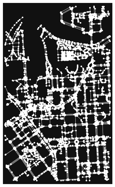
(<Figure size 800x800 with 1 Axes>, <Axes: >)
Note
When exporting to networkx graph, Pyrosm will by default change names of a few variables:
id --> osmid,lon --> x,lat --> y
Also a key column will be added to the edge attributes. This makes it possible to use OSMnx straight away when you export the data. You can distable this behavior by using osmnx_compatible=False in to_graph function.
Calculate shortest paths#
Let’s first see how we can now calculate shortest path between two addresses using networkx and osmnx:
source_address = "Bulevardi 5, Helsinki"
target_address = "Unioninkatu 40, Helsinki"

orig_y, orig_x = ox.geocode(source_address)
dest_y, dest_x = ox.geocode(target_address)
# Print coordinates (lat, lon)
print(orig_y, orig_x)
print(dest_y, dest_x)
60.1650949 24.9388162
60.1723681 24.9503248
Now we need to find the nearest graph nodes for our locations:
# Find the closest nodes from the graph
source_node = ox.distance.nearest_nodes(G, X=orig_x, Y=orig_y)
target_node = ox.distance.nearest_nodes(G, X=dest_x, Y=dest_y)
# Check the nodeids of the source/target node
print(source_node)
print(target_node)
537519894
1012307773
Now it is very easy to calculate the shortest path between those two addresses based on length using networkx function shortest_path(). OSMnx provides very handy function to plot our result on top of the graph:
# Find shortest path (by distance)
import networkx as nx
route = nx.shortest_path(G, source_node, target_node, weight="length")
fig, ax = ox.plot_graph_route(G, route, route_linewidth=6, node_size=0, bgcolor='k')
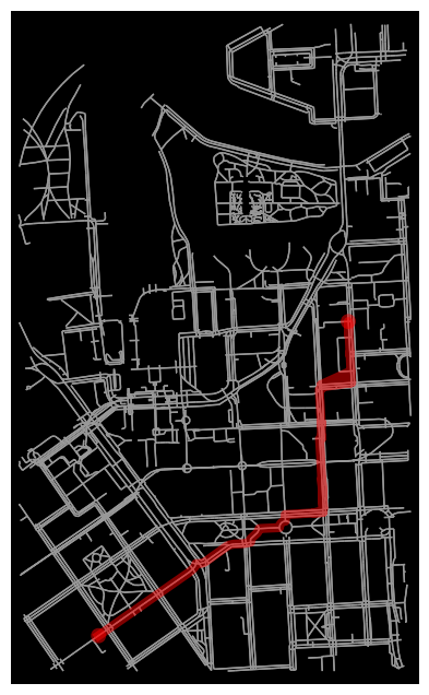
That’s it! Following this approach it is easy to find shortest paths between selected locations.
You can read many more examples from OSMnx examples gallery.
Note
Although NetworkX is very easy to use, it tends to use quite a lot of memory and it is relatively slow with large networks. Hence, the default output graph for pyrosm is iGraph, which performs much better and consumes less memory.
Calculate the catchment areas of hospitals in Estonia with pyrosm + igraph#
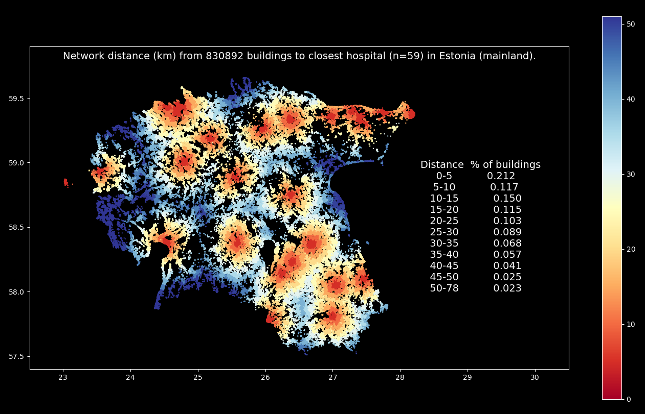
Analyzing the catchment areas of specific services (such as hospitals) is a typical example where large scale spatial network analysis is used. In this example, we will see how pyrosm can be used together with igraph (+ a few other libraries) to conduct large scale network analysis and find the closest hospital for each building in (mainland) Estonia. The whole process should take less than 10 minutes with computer having 16GB of available RAM. The end result will look something like following:
Warning
As OpenStreetMap is a voluntarily maintained data source, the hospitals extracted from OSM might not be up-to-date and some of them might be missing or otherwise incorrect. The hospitals represented in this example can be of any kind (not resticted e.g. to acute care hospitals). Lastly, it would make more sense to assess the number of inhabitants instead of buildings (after all, it’s the people who need care, not the buildings). HOWEVER, the main purpose of this demo is just to give you an idea what can be done, not to make a scientific assessment of health care accessibility in Estonia. If you find a mistake in the OSM data, please contribute and make it better by suggesting an edit at www.openstreetmap.org/
Let’s start by defining a few helper functions for our analysis:
from pyrosm import OSM, get_data
import geopandas as gpd
import pandas as pd
from sklearn.neighbors import BallTree
import numpy as np
import mapclassify as mc
import matplotlib.pyplot as plt
import time

def get_igraph_nodes(G):
    """Retrieves a frame from nodes of the igaph"""
    attributes = G.vs.attribute_names()
    if len(attributes) == 0:
        raise ValueError("Nodes does not have data.")
    data = {name: G.vs[name] for name in attributes}
    if "geometry" in attributes:
        return gpd.GeoDataFrame(data,
                                geometry="geometry",
                                crs="epsg:4326")
    return pd.DataFrame(data)

def get_nearest(src_points, candidates, k_neighbors=1):
    """Find nearest neighbors for all source points from a set of candidate points"""
    tree = BallTree(candidates, leaf_size=15, metric='haversine')
    distances, indices = tree.query(src_points, k=k_neighbors)
    distances = distances.transpose()
    indices = indices.transpose()
    closest = indices[0]
    closest_dist = distances[0]
    return (closest, closest_dist)

def nearest_neighbor(left_gdf, right_gdf, return_dist=False):
    """
    For each point in left_gdf, find closest point in right GeoDataFrame and return them.

    For further info, take a look this lesson:
        https://autogis-site.readthedocs.io/en/latest/notebooks/L3/06_nearest-neighbor-faster.html
    """
    left_geom_col = left_gdf.geometry.name
    right_geom_col = right_gdf.geometry.name
    right = right_gdf.copy().reset_index(drop=True)
    left_radians = np.array(left_gdf[left_geom_col].apply(lambda geom:
                                                          (geom.x * np.pi / 180, geom.y * np.pi / 180)
                                                         ).to_list())
    right_radians = np.array(right[right_geom_col].apply(lambda geom:
                                                         (geom.x * np.pi / 180, geom.y * np.pi / 180)
                                                        ).to_list())
    closest, dist = get_nearest(src_points=left_radians, candidates=right_radians)
    closest_points = right.loc[closest]
    closest_points = closest_points.reset_index(drop=True)
    if return_dist:
        earth_radius = 6371000  # meters
        closest_points['distance'] = dist * earth_radius
    return closest_points

def find_nearest_nodeids(nodes, src_gdf):
    """Finds the nearest node-ids for all points in 'src_gdf'."""
    nearest = nearest_neighbor(src_gdf, nodes, return_dist=True)
    return list(set(nearest["node_id"].values)), nearest["distance"].values
Retrieve the network, buildings and hospitals for Estonia:
# Get the data
osm = OSM(get_data("estonia", update=True))
nodes, edges = osm.get_network(nodes=True, network_type="driving")
hospitals = osm.get_pois({"amenity": ["hospital"]})
buildings = osm.get_buildings()

# Track the number of buildings
building_cnt = len(buildings)
Downloaded Protobuf data 'estonia-latest.osm.pbf' (115.7 MB) to:
'/private/var/folders/f2/pgp09jl542zffhtrt2hx8zhh0000gp/T/pyrosm/estonia-latest.osm.pbf'
Create the directed graph for Estonia:
# Create graph
G = osm.to_graph(nodes, edges)
Get nodes from the graph
This step needs to be done because some of the nodes originally parsed from the street network are likely to be dropped out when the graph is generated (because unconnected edges are removed). Note: you can keep the whole network by specifying
retain_all=Truewhen callingto_graph().
nodes = get_igraph_nodes(G)
Find closest network node for each hospital:
# Ensure that all hospitals are represented as a point (take centroid)
# Warning: using a centroid is not necessarily a smart thing if doing the analysis for real,
# but for the sake of simplicity we assume that the centroid of the hospital polygon
# is the destination to be reached.
hospitals["geometry"] = hospitals.centroid

# Get a list of nearest source-ids of the network to all hospitals (with distance)
# Warning: Using the nearest node (in stead of nearest edge) can produce slightly incorrect results,
# but for the sake of simplicity we use nodes.
src_ids, euclidean_distance = find_nearest_nodeids(nodes, hospitals)
/var/folders/f2/pgp09jl542zffhtrt2hx8zhh0000gp/T/ipykernel_3297/656856640.py:5: UserWarning: Geometry is in a geographic CRS. Results from 'centroid' are likely incorrect. Use 'GeoSeries.to_crs()' to re-project geometries to a projected CRS before this operation.

  hospitals["geometry"] = hospitals.centroid
Calculate travel distances to all hospitals in Estonia:
# Keep track of how many new columns are inserted to the frame
src_cnt = len(src_ids)

# Iterate over hospitals and calculate the network distances
# Note: this could also be run by passing all `src_ids` at once
# to the shortest_paths_dijkstra -function.
for src_id, distance_to_closest_node in zip(src_ids, euclidean_distance):
    #print(f"Calculate shortest paths to {src_id}")

    # Calculate shortest path lengths to given locations
    path_lengths = G.distances(source=src_id, weights="length", mode="IN")

    # Add the euclidean distance between the hospital and closest node in the network
    # to keep track of the door-to-door travel distance
    path_lengths = np.array(path_lengths) + distance_to_closest_node

    # Attach the path lenghts to nodes
    nodes[f"distance_to_{src_id}"] = path_lengths[0]
At this point, we have distance from all nodes in the network to each hospital. They are stored as separate columns in the nodes GeoDataFrame.
Next, we calculate which of the hospitals is the closest one for each node:
# Calculate distance to the closest hospital
nodes["distance_to_closest"] = nodes.iloc[:, -src_cnt:].min(axis=1)

# At this point you could already see the catchment areas from each road network node
# to the closest hospital.
# Comment out the following if you want to see:
# ax = nodes.plot(column="distance_to_closest", cmap="RdYlBu", markersize=0.5)
At this point, we have calculated the catchments for each hospital, but those are not linked yet to buildings.
Let’s find the closest node for each building and keep track of the distance between them:
# Find closest node for each building (centroid)
# Warning: Again, taking a centroid of a building might not be the smartest thing to do for real..
# But for the sake of simplicity, we do it such a way
buildings["centroid"] = buildings.centroid
buildings = buildings.set_geometry("centroid")

# Note: With ~900000 x ~830000 point pairs,
# this takes awhile to solve.
# Also keep track of the distance between the points.
closest = nearest_neighbor(buildings, nodes, return_dist=True)
buildings["node_id"] = closest["node_id"]
buildings["distance_to_closest_node"] = closest["distance"]
/var/folders/f2/pgp09jl542zffhtrt2hx8zhh0000gp/T/ipykernel_3297/519071033.py:4: UserWarning: Geometry is in a geographic CRS. Results from 'centroid' are likely incorrect. Use 'GeoSeries.to_crs()' to re-project geometries to a projected CRS before this operation.

  buildings["centroid"] = buildings.centroid
Now we can associate the distance information to closest hospital into the buildings:
# Link the distance information
access = buildings.merge(nodes[["distance_to_closest", "node_id"]], on="node_id")

# Add the (Euclidean) distance between building
# and the closest node in the road network to get a full "door-to-door" distance
access["distance"] = access["distance_to_closest"] + access["distance_to_closest_node"]

# Calculate distance in kilometers (meters by default)
access["distance_km"] = (access["distance"] / 1000).round(1)
Some of the buildings might be very far from the closest road. Drop buildings that are further than 5km from the road:
# Drop such buildings that are further than 5 km from closest road
access = access.loc[access["distance_to_closest_node"]<=5000]
Notice: the previous step will remove most of the buildings from the islands of Saarenmaa and Hiiumaa, because those are not linked to the mainland network (requires taking a ferry).
Finally, to make things a bit more interesting, we can also classify the distances and calculate some statistics:
# Classify distances to every 2 km zones, specify that the upper boundary is 50 kilometer
# everything above this will be put into a same class
upper_boundary_distance = 50
width = 5

# Use self-defined classification
classifier = mc.UserDefined(access["distance_km"], bins=[x for x in range(0, int(upper_boundary_distance)+1, width)])
access["cls"] = access[["distance_km"]].apply(classifier)
# Replace the class numbers to distance categories (e.g. 0-2, 2-4 .. km etc.)
access["travel_distance"] = access["cls"].replace({k: v
                                                   for k, v in
                                                   zip([x for x in range(len(classifier.bins))],
                                                       classifier.bins)})

# Set all values over 50 km as 51 (to improve how the colorscale works)
access.loc[access["travel_distance"] > upper_boundary_distance, "travel_distance"] = upper_boundary_distance + 1

# Convert the observation counts as percentages
classifier.counts = (classifier.counts / classifier.counts.sum()).round(3)

# Convert stats to dataframe
bins = classifier.bins.astype(int)
categories = np.vstack([bins[:-1], bins[1:]]).T
categories = [f"{low}-{high}" for low, high in categories]
access_zone_classes = pd.DataFrame({"Distance": categories, "% of buildings": classifier.counts[1:]})
Finally, we can plot the results as a map:
plt.style.use('dark_background')
ax = access.plot(column="travel_distance", markersize=0.5, legend=True, cmap="RdYlBu", figsize=(17,10))
# Adjust the map extent
ax.set_xlim(22.5, 30.5)
ax.set_ylim(57.4, 59.9)
# Add some useful info
ax.text(23, 59.8, f"Network distance (km) from {building_cnt} buildings to closest hospital (n={src_cnt}) in Estonia (mainland).", {"size": 14})
ax.text(28.3, 58.0, access_zone_classes.to_string(index=False), {"size": 14});
The map shows the catchment areas of all hospitals in mainland Estonia based on network distance between buildings and the closest hospital. It is possible to spot the 5 kilometer distance zones around each hospital quite easily, and the summary statistics reveal that ~20 % of the buildings in Estonia are within 5 kilometer from the closest hospital, and ~50 % of the buildings in Estonia are within 15 kilometers from closest hospital (however, remember/see the caveats in the beginning of this section about the data quality and the rationale).
This example shows, how pyrosm can be used to conduct even national level analysis quite easily and efficiently. The total time to run this tutorial took about 1.5 minutes (with a laptop having 24GB memory, SSD drive, and Apple M5 processor). This included all steps from downloading the OSM data, parsing the required datasets (steets, buildings and hospitals), exporting the network to graph, conducting the network distance calculations and parsing the statistics (plotting was not taken into account).
Calculate the job accessibility in Helsinki Region with pyrosm + pandarm#
Pandarm (the maintained, NumPy 2-compatible fork of pandana) is a Python network analysis library supported by pyrosm export functionality. Pandarm operates using a fast contraction hierarchies -algorithm and includes various useful functions. In this tutorial, we will see 1) how to calculate distance to nearest 5 restaurants for each network node in the Helsinki Region, and 2) how to calculate a simple job accessibility index for the region based on number of restaurant employees (simulated).
Note
pyrosm also still accepts graph_type="pandana", but pandana is deprecated because it is unmaintained and incompatible with NumPy 2 on Windows. Use "pandarm" (a drop-in replacement with the same API) instead.
from pyrosm import OSM, get_data
import numpy as np
import matplotlib.pyplot as plt
osm = OSM(get_data("helsinki"))
nodes, edges = osm.get_network(network_type="driving", nodes=True)
restaurants = osm.get_pois(custom_filter={"amenity": ["restaurant"]})
G = osm.to_graph(nodes, edges, graph_type="pandarm")
/Users/tenkanh2/Library/CloudStorage/OneDrive-AaltoUniversity/Documents/codes/uni/pyrosm/pyrosm/graphs.py:411: UserWarning: No CRS was passed to geometry input; assuming geographic coordinates
  return _create_pandarm_graph(nodes, edges, from_id_col, to_id_col, weight_cols)
Generating contraction hierarchies with 10 threads.
Setting CH node vector of size 425506
Setting CH edge vector of size 805933
Range graph removed 729278 edges of 1611866
. 10% . 20% . 30% . 40% . 50% . 60% . 70% . 80% . 90% . 100%
# For simplicity, ensure all restaurants are represented as points
restaurants["geometry"] = restaurants.centroid
restaurants = restaurants.dropna(subset=["lon", "lat"])
/var/folders/f2/pgp09jl542zffhtrt2hx8zhh0000gp/T/ipykernel_3297/1294727906.py:2: UserWarning: Geometry is in a geographic CRS. Results from 'centroid' are likely incorrect. Use 'GeoSeries.to_crs()' to re-project geometries to a projected CRS before this operation.

  restaurants["geometry"] = restaurants.centroid
# Precompute distances up to 2000 meters
# Notice using long distance with large network can consume memory quite a bit
G.precompute(2000)
Find nearest X number of POIs for each network node#
After we have done precalculations with pandarm, it allows conducting performant queries, such as querying distances to X number of nearest restaurants for all network nodes.
The following example shows how to find the 5 closest restaurants from each network node (up to 2000 meter distance threshold):
# Attach restaurants to Pandana graph
G.set_pois(category="restaurants", maxdist=2000, maxitems=10,
           x_col=restaurants.lon, y_col=restaurants.lat)
# For each node in the network find distances to 5 closest restaurants (up to 2000 meters)
nearest_five = G.nearest_pois(2000, "restaurants", num_pois=5)
nearest_five.tail(10)
| 1 | 2 | 3 | 4 | 5 | |
|---|---|---|---|---|---|
| 13951328551 | 605.870972 | 963.171997 | 998.500977 | 998.500977 | 1770.901978 |
| 13945837243 | 603.051025 | 960.351990 | 995.681030 | 995.681030 | 1768.082031 |
| 29792020 | 579.440979 | 1009.742004 | 1045.071045 | 1045.071045 | 1817.472046 |
| 13945837247 | 574.932007 | 1005.232971 | 1040.562012 | 1040.562012 | 1812.963013 |
| 7817994382 | 2000.000000 | 2000.000000 | 2000.000000 | 2000.000000 | 2000.000000 |
| 10016653166 | 2000.000000 | 2000.000000 | 2000.000000 | 2000.000000 | 2000.000000 |
| 13638066233 | 2000.000000 | 2000.000000 | 2000.000000 | 2000.000000 | 2000.000000 |
| 13247426322 | 2000.000000 | 2000.000000 | 2000.000000 | 2000.000000 | 2000.000000 |
| 13247426323 | 2000.000000 | 2000.000000 | 2000.000000 | 2000.000000 | 2000.000000 |
| 13247426324 | 2000.000000 | 2000.000000 | 2000.000000 | 2000.000000 | 2000.000000 |
As a result, we get the distance to five nearest restaurants for each node (node-id is the index here).
Calculate the job accessibility#
Next we will use a useful pandarm function called aggregate that allows to calculate accessibility index based on a given numeric variable, such as employee count. Here, we won’t be using any real employee information, but assign a random number of employees for each restaurant (between 1-10). Then we will calculate a specific job accessibility index based on cumulative number of restaurant employees within 500 meters (from each network node). This kind of index can provide a nice overview of the (restaurant) job accessibility in a city.
# Assign a random number of workers for each restaurant (between 1-10)
restaurants["employee_cnt"] = np.random.choice([x for x in range(1,11)], size=len(restaurants))
# Find the closest node-id for each restaurant
node_ids = G.get_node_ids(restaurants.lon, restaurants.lat)
# Add employee counts to the graph
G.set(node_ids, variable=restaurants.employee_cnt, name="employee_cnt")
# Calculate the number of employees (cumulative sum) from each node up to 500 meters
result = G.aggregate(500, func="sum", decay="linear", name="employee_cnt")
result = result.to_frame(name="cum_employees")
# Attach the information from nodes
result = nodes.merge(result, left_on="id", right_on=result.index)
# Visualize the results
plt.style.use('dark_background')
ax = result.plot(column="cum_employees", cmap='BrBG', markersize=0.1, legend=True, figsize=(20, 20))
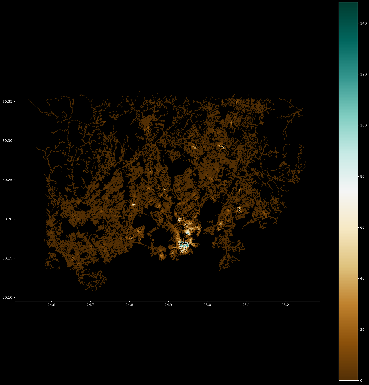
As a result, we get a map showing the restaurant job accessibility in Helsinki Region. The highlighted colors show areas where there are high number of restaurant jobs/employees working (notice that this is not based on real data).