Reading OSM datasets

Once you have a PBF file, the OSM reader turns it into GeoPandas GeoDataFrames. This section shows how to initialise the reader, read the main OSM datasets (street networks, buildings, POIs, landuse, natural elements and boundaries), limit reading to a bounding box, and read historical data.

How to?

• Initialize the OSM reader

• Read street networks

• Read buildings

• Read Points of Interest (POI)

• Read landuse

• Read natural

• Read boundaries

• Read OSM data with a custom filter

• Filter data based on a bounding box

• Read historical OSM data

Initializing the Pyrosm OSM -reader object

When using Pyrosm, the first step is to initialize a specific reader object called OSM that is available from the pyrosm library:

# Import the library
import pyrosm

# Print information about the basic usage of the `OSM` reader object
help(pyrosm.OSM.__init__)

Help on function __init__ in module pyrosm.pyrosm:

__init__(self, filepath, bounding_box=None)
    Initialize self.  See help(type(self)) for accurate signature.

As we can see from the documentation, the OSM object accepts two parameters:

1. filepath which is the filepath to the PBF file (*.osm.pbf) which will be read (see info above how to get one), and

2. bounding_box which is an optional parameter that can be used to filter OSM data geographically from specific area (see here for further details)

The following shows how to initialize an OSM reader object using a test dataset that comes with Pyrosm, and which can be retrieved using a get_data function:

import pyrosm

# Get filepath to test PBF dataset
fp = pyrosm.get_data("test_pbf")
print("Filepath to test data:", fp)

# Initialize the OSM object 
osm = pyrosm.OSM(fp)

# See the type
print("Type of 'osm' instance: ", type(osm))

Filepath to test data: /Users/tenkanh2/Library/CloudStorage/OneDrive-AaltoUniversity/Documents/codes/uni/pyrosm/pyrosm/data/test.osm.pbf
Type of 'osm' instance:  <class 'pyrosm.pyrosm.OSM'>

As we can see, the test dataset lives in my case somewhere under the miniconda3 package, and the type of the osm instance is something called pyrosm.pyrosm.OSM.

Notice that osm (lower case) is the actually initialized reader instance for the given PBF dataset that should always be used to make the calls for fetching different datasets from the OpenStreetMap PBF -file. Read further to see how things work.

Read street networks

Pyrosm makes it easy to filter street networks using the get_network() method. You can parse streets separately for different travel modes by specifying the type of network using network_type -parameter. The allowed network types are:

• walking (default)

• cycling

• driving

• driving+service (includes also public service vehicles)

The following shows how to read all drivable roads from OSM. Notice that from here on, we will import the OSM reader object directly from the package:

from pyrosm import OSM
from pyrosm import get_data

# Pyrosm comes with a couple of test datasets 
# that can be used straight away without
# downloading anything
fp = get_data("test_pbf")

# Initialize the OSM parser object
osm = OSM(fp)

# Read all drivable roads
# =======================
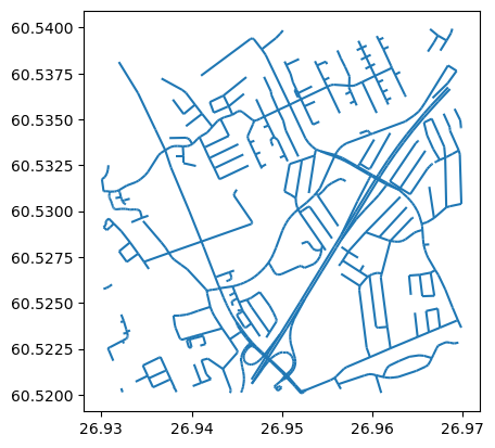
drive_net = osm.get_network(network_type="driving")
drive_net.plot()

<Axes: >

The network contains various information that is parsed from the OSM data, and includes length column that contains information about the length of the road in meters (scroll right):

drive_net.head(2)

	access	bridge	highway	int_ref	lanes	lit	maxspeed	name	oneway	ref	service	surface	id	timestamp	version	tags	osm_type	geometry	length
0	NaN	NaN	secondary	NaN	2	NaN	80	Hurukselantie	NaN	357	NaN	asphalt	4732994	1441800394	23	{"visible":false,"name:fi":"Hurukselantie"}	way	MULTILINESTRING ((26.9431 60.5258, 26.94295 60...	1504.0
1	NaN	NaN	secondary	NaN	NaN	NaN	NaN	NaN	yes	170	NaN	NaN	5184588	1378828296	7	{"visible":false}	way	MULTILINESTRING ((26.94778 60.52231, 26.94717 ...	242.0

Notice that each way in the network is represented as a MultiLineString geometry constructed from multiple road segments. This is how the data is represented by default in OSM. However, this differs if reading nodes and edges: in that case each road segment is represented as a separate row in data (to improve connectivity).

Hint

It is also possible to export network to routable graphs in various formats using to_graph() function (new in version 0.6.0). Read more from “Export street networks to graph -section”.

Understanding the “osm_type” -column values

pyrosm will create a column osm_type to the result which can contain values node, way or relation. These correspond to the three basic components of OpenStreetMap’s conceptual data model of the physical world:

• nodes (points in space),

• ways (linear features and area boundaries),

• relations (sometimes used to explain how other elements work together).

Hence, the “way” values in osm_type column might not necessarily represent only LineString features, as they can also be Polygons or LinearRings. If you want to know the geometry types of your data, you can access such information with geopandas by calling (gdf here represents a GeoDataFrame): gdf["geometry_types"] = gdf.geom_type

Check an example here to see how to filter your GeoDataFrame based on specific geometry type.

Read buildings

from pyrosm import OSM
from pyrosm import get_data
fp = get_data("test_pbf")
# Initialize the OSM parser object
osm = OSM(fp)
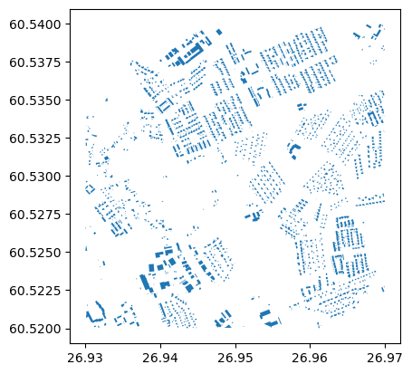
buildings = osm.get_buildings()
buildings.plot()

<Axes: >

Read Points of Interest

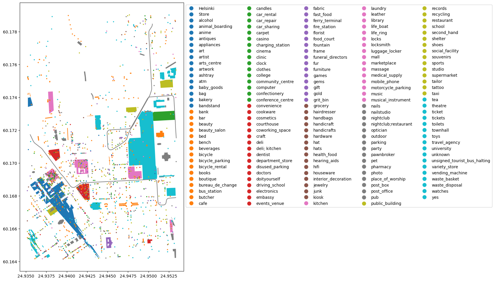
# Read POIs such as amenities and shops
# =====================================
from pyrosm import OSM
from pyrosm import get_data
fp = get_data("helsinki_pbf")
# Initialize the OSM parser object
osm = OSM(fp)

# By default pyrosm reads all elements having "amenity", "shop" or "tourism" tag
# Here, let's read only "amenity" and "shop" by applying a custom filter that
# overrides the default filtering mechanism
custom_filter = {'amenity': True, "shop": True}
pois = osm.get_pois(custom_filter=custom_filter)

# Gather info about POI type (combines the tag info from "amenity" and "shop")
pois["poi_type"] = pois["amenity"]
pois["poi_type"] = pois["poi_type"].fillna(pois["shop"])

# Plot
ax = pois.plot(column='poi_type', markersize=3, figsize=(12,12), legend=True, legend_kwds=dict(loc='upper left', ncol=5, bbox_to_anchor=(1, 1)))

Read landuse

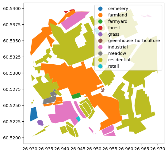
# Read landuse
# ============
from pyrosm import OSM
from pyrosm import get_data
fp = get_data("test_pbf")
# Initialize the OSM parser object
osm = OSM(fp)
landuse = osm.get_landuse()
landuse.plot(column='landuse', legend=True, figsize=(10,6))

<Axes: >

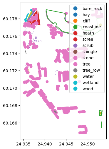
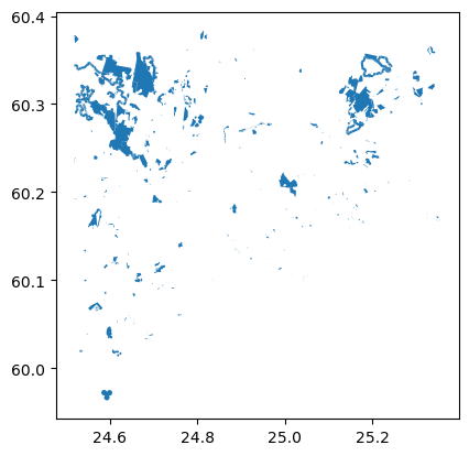
Read natural

# Read natural
# ============
from pyrosm import OSM
from pyrosm import get_data
fp = get_data("helsinki_pbf")
# Initialize the OSM parser object
osm = OSM(fp)
natural = osm.get_natural()
natural.plot(column='natural', legend=True, figsize=(10,6))

<Axes: >

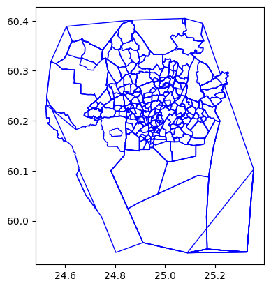
Read boundaries

Pyrosm supports reading boundaries such as administrative borders from PBF using get_boundaries() -function. By default, the function reads all "administrative" borders from the PBF. You can adjust the type of boundary that is parsed from PBF by modifying boundary_type -parameter. You can also search boundaries for specific name using name parameter:

from pyrosm import OSM
from pyrosm import get_data
fp = get_data("helsinki_region_pbf")
osm = OSM(fp)

# Read all boundaries using the default settings
boundaries = osm.get_boundaries()
boundaries.plot(facecolor="none", edgecolor="blue")

Downloaded Protobuf data 'Helsinki_region.osm.pbf' (34.99 MB) to:
'/var/folders/f2/pgp09jl542zffhtrt2hx8zhh0000gp/T/pyrosm/Helsinki_region.osm.pbf'

<Axes: >

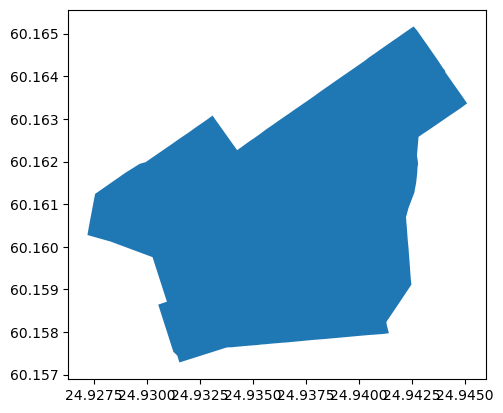
The following shows how to search a specific boundary using the name -parameter.

# Note: the following uses the same osm instance initialized above
selected_boundary = osm.get_boundaries(name="Punavuori")
selected_boundary.plot()

<Axes: >

The name search functionality supports partial text search, meaning that e.g. a query "vuori" would return all elements where the work "vuori" is included in the name tag (such as “Punavuori”):

# Use a partial name "vuori" to look for data
selected_boundary = osm.get_boundaries(name="vuori")
selected_boundary.plot()

<Axes: >

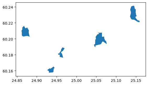
As we can see there were multiple boundaries in the data that included the word "vuori" in their name:

# Check all records that have the word "vuori" in their name
selected_boundary['name'].unique()

<StringArray>
['Punavuori', 'Munkkivuori', 'Roihuvuori', 'Mustavuori', 'Vilhonvuori']
Length: 5, dtype: str

It is also possible to search different kind of boundaries from the PBF.

Supported boundary types are:

• "administrative (default)

• "national_park"

• "political"

• "postal_code"

• "protected_area"

• "aboriginal_lands"

• "maritime"

• "lot"

• "parcel"

• "tract"

• "marker"

• "all"

Let’s read all "protected_area" boundaries from the PBF:

# Note: the following uses the same osm instance initialized above 
protected_areas = osm.get_boundaries(boundary_type="protected_area")
protected_areas.plot()

<Axes: >

Read OSM data with custom filter

Pyrosm also allows making custom queries. For example, to parse all transit related OSM elements you can use following approach and create a custom filter combining multiple criteria:

from pyrosm import OSM
from pyrosm import get_data
fp = get_data("helsinki_pbf")

# Initialize the OSM parser object with test data from Helsinki
osm = OSM(fp)

# Test reading all transit related data (bus, trains, trams, metro etc.)
# Exclude nodes (not keeping stops, etc.)
routes = ["bus", "ferry", "railway", "subway", "train", "tram", "trolleybus"]
rails = ["tramway", "light_rail", "rail", "subway", "tram"]
bus = ['yes']
transit = osm.get_data_by_custom_criteria(custom_filter={
                                        'route': routes,
                                        'railway': rails,
                                        'bus': bus,
                                        'public_transport': True},
                                        # Keep data matching the criteria above
                                        filter_type="keep",
                                        # Do not keep nodes (point data)    
                                        keep_nodes=False, 
                                        keep_ways=True, 
                                        keep_relations=True)
transit.plot()

<Axes: >

Further information on how to make customized queries is available in Parsing OSM data with custom queries.

Filtering data based on bounding box

Quite often one might be needing to extract only a subset of the whole OSM PBF file covering e.g. a specific region. Pyrosm provides an easy way to filter even larger PBF files using a bounding box (rectangular shape) or a more complex geometric feature (e.g. a Polygon). In the following, we will go through the process of extracting a small sample from the whole PBF dataset for specific area of interest. We will use a data dump from Greater London region and extract data covering the Borough of Camden.

from pyrosm import OSM, get_data

# Download a dataset for Greater London (update if exists in the temp already)
fp = get_data("Greater London", update=True)
osm = OSM(fp)

Downloaded Protobuf data 'greater-london-latest.osm.pbf' (55.49 MB) to:
'C:\Users\hentenka\AppData\Local\Temp\pyrosm\greater-london-latest.osm.pbf'

# Read buildings (takes ~30 seconds)
buildings = osm.get_buildings()
buildings.head(2)

	addr:city	addr:country	addr:full	addr:housenumber	addr:housename	addr:postcode	addr:place	addr:street	email	name	...	source	start_date	wikipedia	id	timestamp	version	tags	geometry	osm_type	changeset
0	None	None	None	None	None	None	None	None	None	Laurence House	...	None	None	None	2956186	1469657765	2	None	POLYGON ((-0.02162 51.44472, -0.02033 51.44469...	way	NaN
1	None	None	None	None	Town Hall	SE6 4RU	None	Catford Broadway	None	Lewisham Town Hall	...	None	None	None	2956187	1504282380	5	None	POLYGON ((-0.02110 51.44523, -0.02132 51.44508...	way	NaN

2 rows × 41 columns

# Plot the buildings (will take awhile to plot)
buildings.plot()

<matplotlib.axes._subplots.AxesSubplot at 0x1c18de4b9c8>

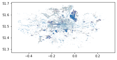
Now have parsed quite a few buildings from the Greater London area (~488,000).

Let’s filter the data spatially and include only buildings from the Borough of Camden. There are a couple of ways how you can pass the bounding box information to the Pyrosm:

1. You can specify the bounding box by a list of x- and y-coordinates (in decimal degrees) of the lower left corner and upper right corner of the geographical area (rectangular) that you want to keep as a result: [minx, miny, maxx, maxy]

2. You can also specify the bounding by passing a Shapely Polygon, MultiPolygon or LinearRing (all closed geometries supported) that can be used to filter the data with a more complex geographical features.

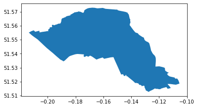
We will now use the boundary of the Camden Borough as our spatial filter. For finding the boundaries of Camden Borough is easy by utilizing the get_boundaries() -function and using the name parameter:

# Get the borough of Camden as our bounding box
bounding_box = osm.get_boundaries(name="London Borough of Camden")
bounding_box.plot()

<matplotlib.axes._subplots.AxesSubplot at 0x1c2a2d6e588>

Now we can initialize the OSM reader with the given bounding box that will then keep the data only from the areas that are within the given bounding box:

# Get the shapely geometry from GeoDataFrame
bbox_geom = bounding_box['geometry'].values[0]

# Initiliaze with bounding box
osm = OSM(fp, bounding_box=bbox_geom)

Now the bounding box information is stored in the attribute bounding_box that will be applied every time when an extract of the PBF (e.g. buildings, roads, etc.) is parsed:

# Bounding box is now stored as an attribute 
osm.bounding_box

Finally, let’s read the buildings now from the Camden Borough using our bounding box filter. Notice, that you do not need to make any changes to the actual get_buildings() call, as the bounding box information is read automatically from the osm instance (osm.bounding_box).

# Retrieve buildings for Camden
camden = osm.get_buildings()

Okay, now we have data for the Camden area! Let’s take a look what it looks like on a map. Here, we will color the building based on how it has been tagged in the OSM:

# Let's plot the buildings and specify colors according the type of the building
ax = camden.plot(column="building", figsize=(12,12), legend=True, legend_kwds=dict(loc='upper left', ncol=3, bbox_to_anchor=(1, 1)))

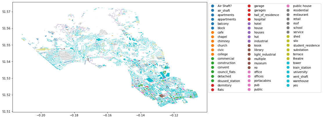
Great, now we can see that a subset of the data was taken according our bounding box coordinates.

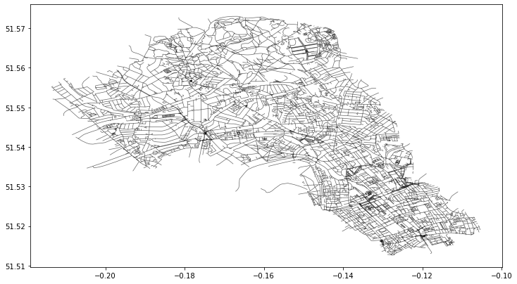
We can utilize the same bounding box for filtering other datasets as well, which can be handy. Let’s also filter the walkable roads from the same area:

# Apply the same bounding box filter and retrieve walking network
walk = osm.get_network("walking")
walk.plot(color="k", figsize=(12,12), lw=0.7, alpha=0.6)

<matplotlib.axes._subplots.AxesSubplot at 0x1c1ecc78088>

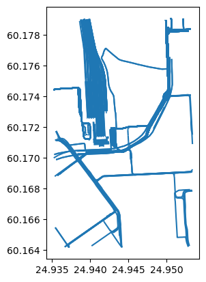
Read historical OSM data

So far we have read data from regular .osm.pbf files, which contain a single snapshot of OpenStreetMap — the data as it looked at the moment the extract was made. OpenStreetMap also publishes history files (.osh.pbf), which keep every version of every element, together with the timestamp at which each version was edited. With a history file you can read the data as it looked at any chosen moment in time, which is useful for studying how an area has changed.

pyrosm recognises a history file automatically from its filename: as long as the path contains osh.pbf, the reader switches into history mode. You can then pass a timestamp to any of the get_* methods to choose the moment you want.

Note: History files for whole regions can be downloaded from Geofabrik, but those downloads require logging in with an OpenStreetMap account, so pyrosm cannot fetch them for you. You point pyrosm at a file you have downloaded yourself. For this example we use a small bundled sample of central Helsinki.

Let’s start by downloading the sample history file and initialising the reader:

from pyrosm import OSM, get_data

# Download a small sample history file for Helsinki
fp = get_data("helsinki_history_pbf")

# Initialise the reader; pyrosm detects the .osh.pbf file as a history file
osm = OSM(fp)

Downloaded Protobuf data 'Helsinki-sample.osh.pbf' (12.75 MB) to:
'/var/folders/f2/pgp09jl542zffhtrt2hx8zhh0000gp/T/pyrosm/Helsinki-sample.osh.pbf'

Now we can read the driving network as it looked at a chosen moment by passing a timestamp. The timestamp is interpreted in UTC and can be given either as a full date and time or as a date alone (in which case midnight at the start of that day is used):

# Read the driving network as it was at the start of 2019
net_2019 = osm.get_network(network_type="driving", timestamp="2019-01-01")
print(f"Edges in the 2019 snapshot: {len(net_2019)}")

Edges in the 2019 snapshot: 7267

For each element, pyrosm selects the most recent version edited up to the timestamp you gave. An element can therefore be older than the timestamp — its latest edit is kept — but versions edited after the timestamp are ignored. Elements that did not yet exist at that moment are left out entirely.

Let’s read a later snapshot of the same network and compare:

# Read the same network as it was at the start of 2021
net_2021 = osm.get_network(network_type="driving", timestamp="2021-01-01")
print(f"Edges in the 2021 snapshot: {len(net_2021)}")

Edges in the 2021 snapshot: 8348

Here we see how the network in this part of Helsinki has changed between the two dates: the 2019 snapshot has 7,267 edges and the 2021 snapshot has 8,348, as mappers added and edited roads over time. A later snapshot typically contains at least as many features as an earlier one. By varying the timestamp you can reconstruct the state of the data at any point covered by the history file.

Be careful: if you read from an .osh.pbf file without giving a timestamp, pyrosm falls back to the current UTC time and emits a warning, since there is no single “current” snapshot in a history file. It is important to understand what this fallback actually returns: it selects the most recent version of each element that is present in the file. A history file is a static download — it only contains edits up to the moment it was produced — so “the current time” does not give you today’s live OpenStreetMap data, but the latest state captured in that particular file. The bundled Helsinki sample, for example, was produced back in 2021, so reading it without a timestamp reflects the situation in 2021, not the present day. Always pass an explicit timestamp when you read historical data, both so that your results are reproducible and so that it is clear which moment in time they represent.